Important features

Command line access

As expressed above, DS9 will execute a Shell command, which will call the package's functions. DS9 allows prompting this command each time a function is launched through: Analysis -> Analysis command log. Copy-pasting this command into a Shell interpreter (like Terminal) will provide the same result. The package is then totally accessible via a Shell interpreter via command lines.

This important feature could allow the plugin to be operated from other image visualization software like Ginga or Glueviz. Running DS9Utils inside the terminal will show all the available functions and running DS9Utils <function> -h will display the help of the related function. This leads to the next major feature: multi-image analysis.

All functions arguments are parsed through the argparse module. Functions can then be called from DS9, terminal or directly from Python using argv parameter: \(\verb! Python_command(argv="-p '/data/**/*.fits' -e 'ds9-=1'")! \label{eq:Python}\)

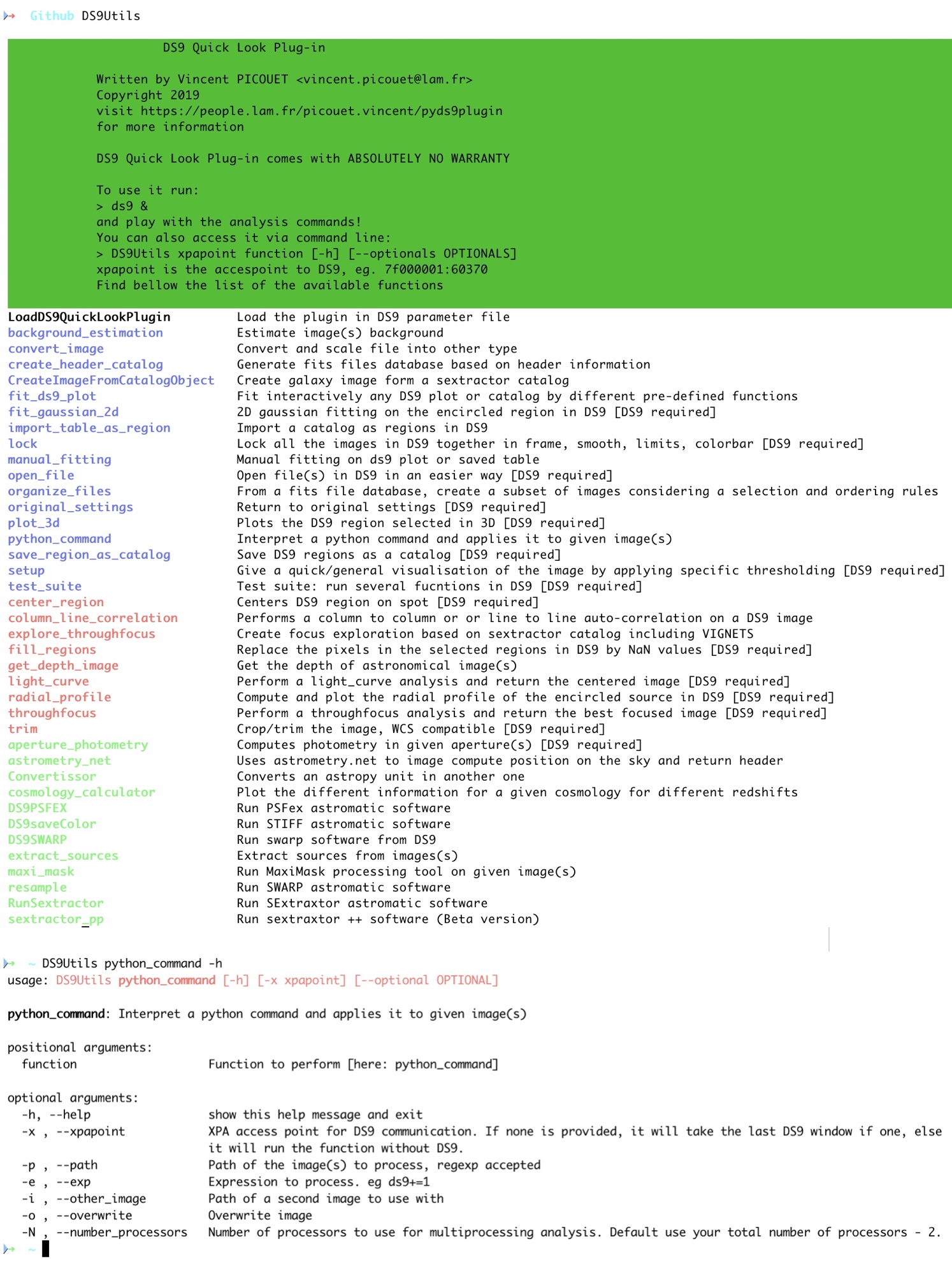Command-line interface of DS9Utils. Calling DS9Utils, display all the available functions. Calling a specific function with -h argument displays the help and the functions parameters.

Multi-image and multi-threaded analysis

pyds9plugin is, in essence, a quick-look plugin that is perfect for visualizing, exploring, analyzing, and processing the displayed image. However, it was essential to make it suitable for more important pipelines as soon as the parameters have been tuned. To this end, all processing functions can be launched on a set of images by specifying the path of all the images using regular expression:

DS9Utils <function> [-o OPTIONAL] --path "/data/**/*.fits"

This feature allows, for instance, to spend important time optimizing interactively the \(\sim50\) parameters of source extraction and add a whole image folder to the analysis command to process all the images when the parameters have been fine-tuned.

To take advantage of modern computer architectures, it uses multi-threading to run each image on a different thread. The number of processors to be used is accessible via -N or --number_processors argument. By default, the code will use the total number of processors of the machine minus 2. A video can be found .

Python interpreter

We added a Python interpreter to the extension. This allows directly applying Pythonic one-line transformations to the displayed image.

We list below some of the numerous one-line possibilities that can, for instance, be used for generating some noise images, apply linear transformation to images to decrease artificially your exposure time for instance), add noise to your image, mask bright sources, or perform more complex transformations like fast Fourier transform or auto-correlation.

DS9 = np.median(ds9) + 0.1 (ds9-np.median(ds9))

ds9+=np.random.normal(0,0.5*ds9.std(),size=ds9.shape)

ds9+=np.random.normal(0,0.5*ds9.std(),size=ds9.shape)

ds9[ds9>np.percentile(ds9,99)]=np.nan

ds9=abs(fftshift(fft2(ds9)))**2

ds9=correlate2d(ds9,ds9,boundary='symm', mode='same')

Python macros

Because one line is short, it is possible to simply give the path of a Python file. For instance, giving the path of the code below interpolates masked values in the DS9 frame and returns the new image in the DS9 GUI:

\ Basically, any function that does not require user's parameters can be directly implemented this way which is simpler as multiprocessing is already implemented. As well as for the previous section, the defined function can be run on a set of images by adding the regular expression path to the --path parameter (see Section 3.1.2 and ):

DS9Utils python_command --exp "/softs/pipe.py" -p "/data/**/*.fits"

The different variables that can be used inside macros are ds9 for the image loaded in DS9 and header for its header and d is the XPA access point for a more extensive communication with DS9.

Following lessons learned from @Joye2005, I decided to include in DS9 analysis functions only the ones that are generic/helpful and that require input parameters. Functions that do not require any parameter should be implemented as macros as multiprocessing is already implemented. To help people write their own, I published within the plugin several macros (in DS9functions/macros). Each macro (FFT.py, Autocorrelation.py, trimming.py, Column_line_correlation.py, Interpolate_NaNs.py, etc.) can either contain one specific task (compute and return the FFT of the DS9 image, trim wcs images, interpolate masked values in the image, etc.) or a series of processing (background subtraction source extraction astrometric calibration)

from astropy.convolution import interpolate_replace_nans, Gaussian2DKernel

STD_DEV = 1
while ~np.isfinite(ds9).all():
  kernel = Gaussian2DKernel(x_stddev=STD_DEV, y_stddev=STD_DEV)
  ds9 = interpolate_replace_nans(ds9, kernel)
  STD_DEV += 1

VTK 3D rendering

The Visualization Toolkit (VTK) is the leading open-source software for manipulating and displaying scientific data. It comes with state-of-the-art tools for 3D rendering, a suite of widgets for 3D interaction, and is already supported by some of the other applications (JS9, Icy, AstroImageJ). We integrated it into the plugin to increase the interaction with selected regions in the image. The function allows to add contours, smooth the image rendering, change the scale, or create a rotating .gif video. Possibility to even fit interactively 2D Gaussians. It is also possible to analyze time series in 3D like through-focus or to explore the focus in the field.

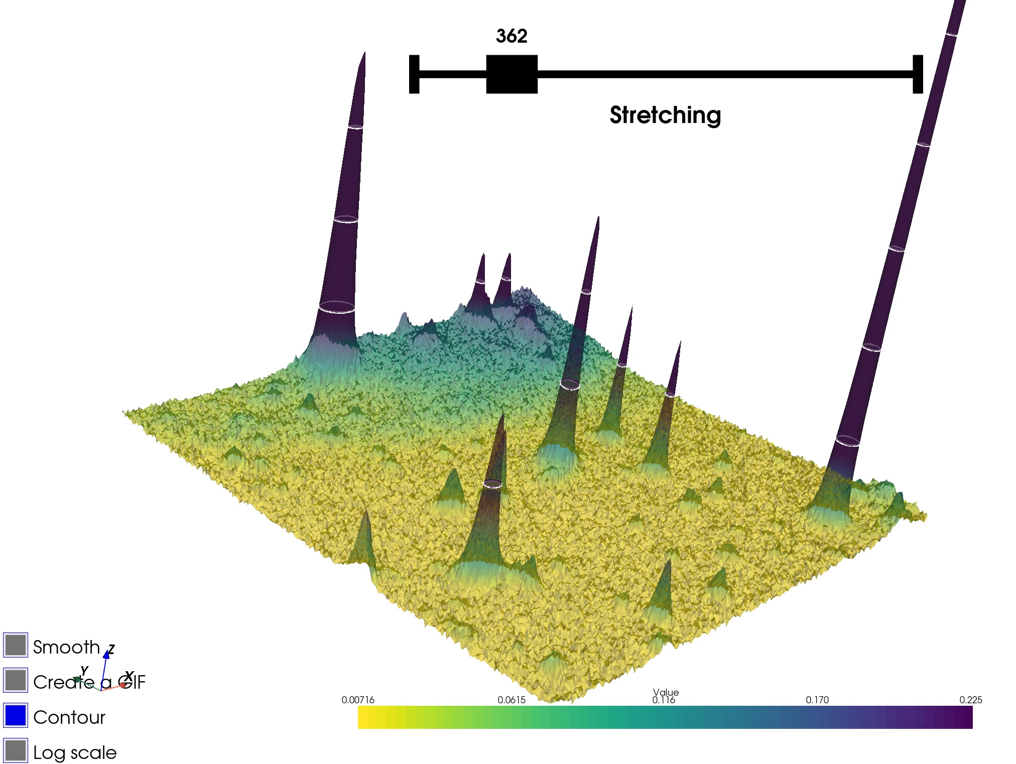3D VTK rendering: the different widgets in the bottom left corner allow to interact with the plotter and create animated GIFs. 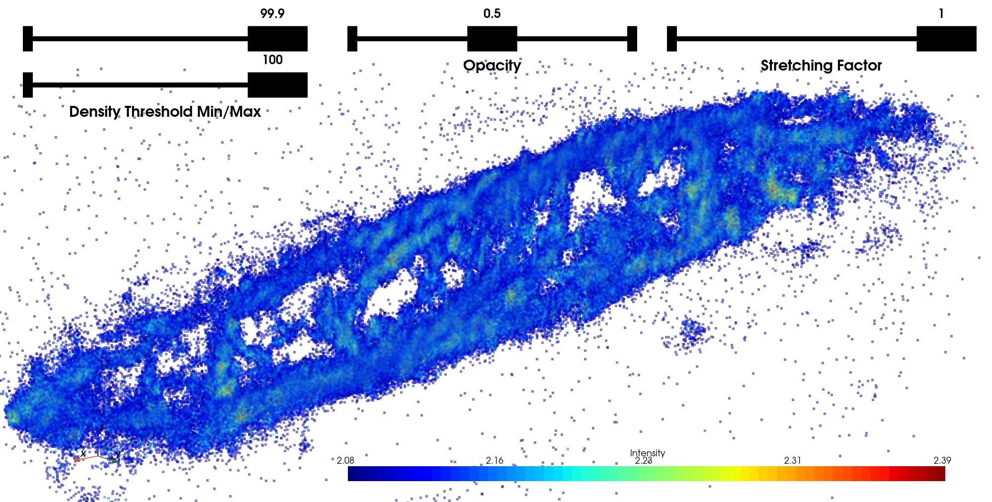3D VTK rendering: the different widgets in the top allow to interact with the plotter and create animated GIFs.

Interactive profile fitting

DS9 incorporates the very useful possibility to interactively plot 1D profiles (can be tilted, stacked in the orthogonal direction, plot the third axis component, etc). This gives essential qualitative information.

Because it is essential to retrieve information from images (spatial/spectral resolution, diffusion exponential decay, etc.) it is critical to turn this qualitative information into re-usable quantitative information. To do this we added an interactive plot fitter to the extension (based on the dataphile package). This allows fitting 1-D profiles with interactive adjustment of the initial guess parameters to ensure that the fit converges. This function works on any DS9 plot, which means that plots generated via the plugin (radial profile or light curve) can be fitted with this function.

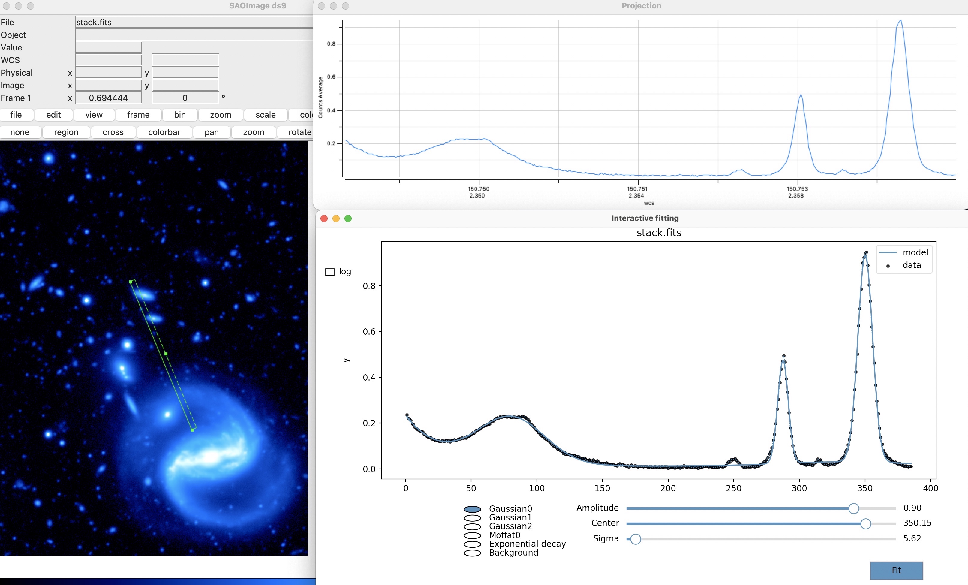
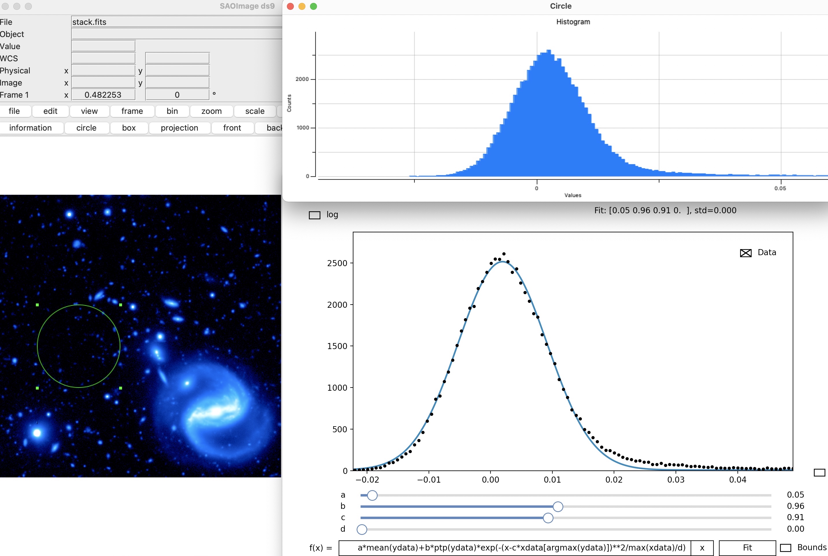
As multi-feature analysis is essential in astronomy, the fitting is decomposed into two components: the background and the features added to the background. The different background possibles are constant, slope, exponential, double-exponential, logarithmic. It is then possible to add any number of features among Gaussian, Voigt, or Moffat profiles (see Figure [ds9/fit2d.jpg] ). Each feature parameter can be moved independently to be sure that the final fit converges. The definition of the different functions is shown in table 1. To get the most of this fitting function, we added the possibility to add any other user-defined functions.

The function just needs to be added to the package file:\ pyds9plugin/Macros/Fitting_Functions/functions.py

For each fitted parameter, be sure to define a list as default argument as it will be used to define the lower and upper bounds of the widget fitter.

Function	Formula
Constant	\(y = a\)
Slope	\(y=a \times x\)
Exponential	\(y=a\times e^{-\frac{x}{b}}\)
Logarithmic	\(y=a + b\times ln(x-c)\)
Double exponential	\(y=a\times e^{-\frac{x}{b}} + c\times e^{-\frac{x}{d}}\)
Gaussian	\(y=a \times e^{-(\frac{c-b}{2*c})^2}\)
Moffat	\(y=a\times (1 + \frac{x-b}{c}^{2})^{-d}\)
Voight	\(y=a \times\frac{ \mathbb{R}\left ( wofz \left ( \frac{(x-b) \gamma i}{c\sqrt{\pi}} \right ) \right ) }{ \mathbb{R}\left ( wofz \left ( \frac{x \gamma i}{c\sqrt{\pi}} \right ) \right ) }\)

Fitting functions of the profile fitter. The first four functions are the possible backgrounds to fit. On top of this background, you can add as many Gaussian/Moffat/Voigt features as you want. The wofz function in the last line is the Faddeeva function \(wofz(z)=e^{-z^2} \times (1-erf(-iz) )\) accessible in Python via scipy.special.wofz

If no plot neither catalog is given, the window will work as a regular plotter, where the user can plot its own function and change the parameters.

Fits file organizer

This final functionality is a fits organizer, divided into two functions (Create header database and Filtering and organizing images). The first function generates from the input images (regular expression) a catalog (CSV table) concatenating all information contained in the header images. It will also add important information such as the path, directory, basename, creation and modification date, size, etc. of each image.

The output database will give at a glance all image information which will help understand the dataset, spot failures in the acquisition, etc. It can also be open with TOPCAT to perform more complex analysis and selection of images.

As only header information is read (not the pixels), the function is fast even on a significant number of files (a few seconds for thousands of files). Still, it can be very interesting to add to the output header catalog some image information such as the images' median, noise, the number of saturated pixels, or any other information. To this end, the function accepts Header catalog Macros where the user can write any Python command to append image estimators to the output header catalog. For instance, the following piece of code add to the header database some information about the image (column/line correlation, saturated pixels fraction, number of cosmic rays, etc.):

import numpy as np

SATURATION = 2 ** 16 -1
data = fitsfile[0].data
columns = np.nanmean(data, axis=1)
lines = np.nanmean(data, axis=0)
table['median'] = np.nanmedian(data)
table["Lines_difference"] = np.nanmedian(lines[::2]) - np.nanmedian(lines[1::2])
table["Columns_difference"] = np.nanmedian(columns[::2]) - np.nanmedian(columns[1::2])
table["SaturatedPixels"] = 100 * np.mean(data > SATURATION)
table["CosmicRays"] = count_cosmic_rays(data)

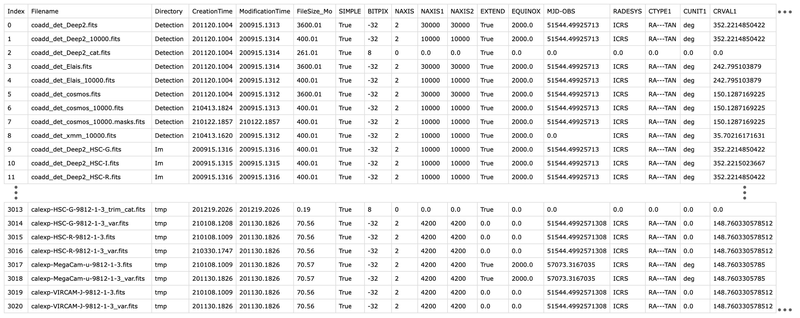Output header database of the 3021 images contained in Home. Combining it with a Python script adding image information would only attach additional information to this table.

The output header database can be used with the second function, which filters the images and organizes them following organizational rules. This function allows creating subsets of images verifying some header conditions. For instance, all images created after the 12th of September 2020 that have a positive EMGAIN or an exposure higher than 100 seconds can be recovered with this condition: \(\renewcommand{\theequation}{6} \verb! (EMGAIN > 0 | EXPOSURE >100) & CreationTime>200912 ! \label{eq:selection}\)

The files are then directly organized in the file system with an arborescence following the column names. For instance, by giving EMGAIN,EXPOSURE, all files will get organized as shown in next figure. The function only generates aliases and does not move any original files. The header database and organized aliases are respectively saved in ~/DS9QuickLookPlugIn/HeaderDataBase and ~/DS9QuickLookPlugIn/subsets.

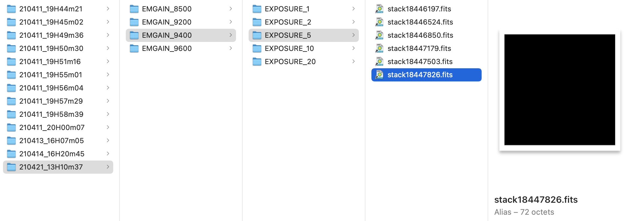Fits file organization following the previous selection and the organization rule EMGAIN,EXPOSURE.